install.packages("usethis")
usethis::use_blank_slate()R Recap Before the Lab Exam
Introduction to Quantitative Methods · Sciences Po
Lennart Klein
19 November 2026
Today
By the end you should have
- an RStudio project you can reuse
on Tuesday - a feel for how R reads a line of code
- a routine for fixing errors, with or
without AI
The idea of this session
- code along and interrupt with any questions
- everything builds on TAs’ labs and the lecture
- I am just a nerd who likes to share R <3
- slides are recycled from my time as a TA
1 · Setting Up a Project
and RStudio
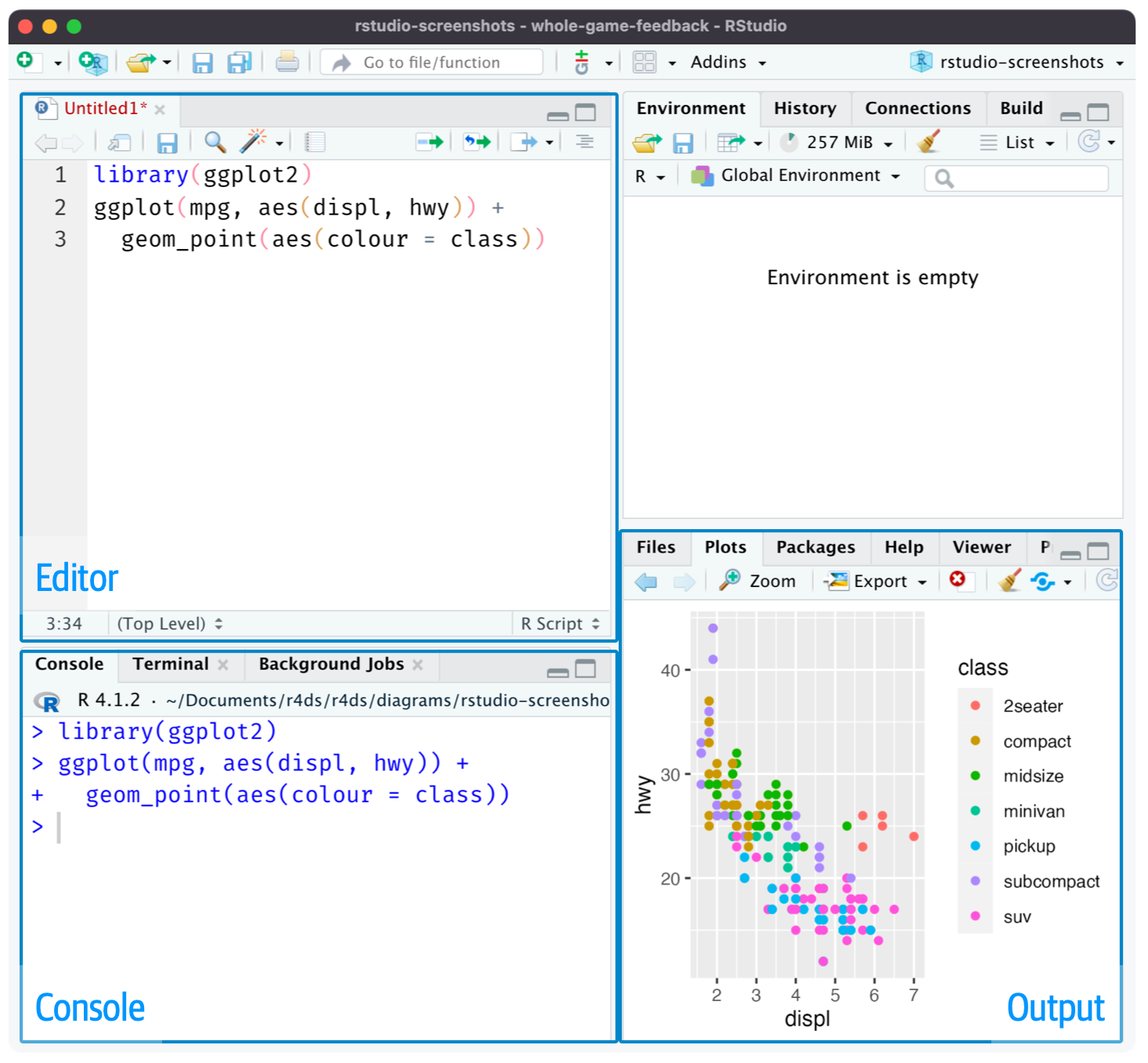
Figure: Wickham et al., R for Data Science (2e), CC BY-NC-ND 3.0
R does the statistics. RStudio is where you write it.
- Editor: your script, the file you hand in
-
Console: runs R.
>ready,+unfinished line - Terminal: not R, only for setup
- Environment: data objects & variables in memory
- Output: plots, help, files
Best Practice: One folder per project
A good folder structure (example):
labexam/
├── labexam.Rproj    ← double-click this
├── data/
│   ├── anes_….csv
│   └── ess.csv
├── output/
└── Lastname_Firstname.R- In RStudio, create one with:
File > New Project > New Directory. - Opening
labexam.Rprojautomatically makes this folder the working directory. -
read.csv("data/ess.csv")then works on any computer, withoutsetwd(). - [TIP] Before you hand in:
Session > Restart R, then run the whole script again to make sure it works.
Best Practice: Start every session from a clean slate
By default, RStudio saves everything in memory to .RData when you quit and loads it again next time. Yesterday’s objects come back, and a script can seem to work only because of them.
Tools > Global Options > General:
- untick Restore .RData into workspace at startup
- set Save workspace to .RData on exit to Never
Or run this once in the Console:
Your script is what counts. To test it: Session > Restart R (Cmd+Shift+0 on a Mac, Ctrl+Shift+F10 on Windows), then run everything from the top.
The top of your script might look something like this
Install the packages once, in the Console (not in the script):
install.packages(c("dplyr", "lmtest", "car", "margins", "nnet"))2 · How R Reads Code
Three patterns you see in every lab script
| Pattern | Read it as | Example |
|---|---|---|
name <- value |
“name gets value” | x <- c(3, 7, 10) |
function(arguments) |
“do this, with these settings” | mean(x, na.rm = TRUE) |
dataset$var |
“the column var of dataset” | dataset$agea |
A condition gives TRUE or FALSE for every row
ifelse() is Excel’s IF() for every row
    0     1     2     3     4     5     6     7     8     9    10  <NA>
 1318   775  2005  3522  3339 11259  3360  3711  2852   928  1371  5074
useNAcontrols if the table includes counts ofNAvalues: the allowed values correspond to never ("no"), only if the count is positive ("ifany") and even for zero counts ("always"). (?table)The default is
"no", which would hide the 5,074 newNAs.
One NA makes the result NA
Packages
install.packages("car") |
downloads it, once per computer |
library(car) |
loads it, in every session |
car::vif(model) |
uses one function without library()
|
If R says could not find function "vif", load the package with library(car).
If it says there is no package called 'car', install it first.
Base R functions such as mean, lm and t.test are always available.
Base R and the tidyverse
Base R, as in the labs:
dplyr, with the native pipe |> (“then”):
dataset <- dataset |>
  mutate(
    age_cat = case_when(
      age <= 30 ~ 0,
      age <= 60 ~ 1,
      age >= 61 ~ 2
    )
  )
The Lab 3 solution writes the older pipe %>% (from the magrittr package), which does the same here. Both versions give the same variable. Wajd: “THEY WORK THE SAME WAY, so use whichever one you prefer.” Base R is closer to the lab scripts, which helps on Tuesday.
y ~ x means “y explained by x”
The same formula works in five functions from the labs:
# means by group
aggregate(lrscale_clean ~ gndr, data = dataset, FUN = mean)

# difference of means
t.test(lrscale_clean ~ gndr, data = dataset)

# figure
boxplot(lrscale_clean ~ gndr, data = dataset)

# regression
lm(lrscale_clean ~ age + factor(gndr) + edu, data = dataset)

# logistic regression (y01 is a 0/1 dummy variable)
glm(y01 ~ age + factor(gndr), data = dataset, family = binomial)
+adds a predictor.*adds two predictors and their interaction.
factor(): numbers that are labels
  (Intercept) factor(gndr)2
5.2665148 -0.2946513 -
gndrcodes 1 = male and 2 = female, so the numbers are categories, not amounts. -
factor(gndr)2compares women with men. Men are the reference: the first level, which gets no row of its own. -
factor(cntry)adds one dummy per country, compared with AT (first in alphabetical order). These are the country fixed effects.
3 · From Output to Words
Describe a variable (Lab 2)
mean(anes$like_democrat, na.rm = TRUE)[1] 4.87644median(anes$like_democrat, na.rm = TRUE)[1] 5sd(anes$like_democrat, na.rm = TRUE)[1] 3.405986Given that the mean and the median are very close, the distribution of the rating of the Democratic Party is approximately symmetric. The standard deviation means that ratings typically lie about 3.4 points from the mean, which is large compared with the mean: the spread of the distribution is thus large.
Histogram (Lab 2)
hist(anes$like_democrat)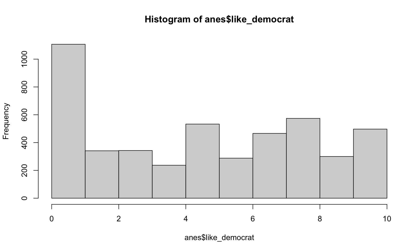
The bars show the shape that the mean and median describe. The first bar counts the 0s and the 1s together; breaks = seq(-0.5, 10.5, by = 1) gives one bar per value.
Group means (Lab 2)
aggregate(like_democrat ~ voted_2024, data = anes, FUN = mean) voted_2024 like_democrat
1 0 4.373077
2 1 4.949704Non-voters: 4.37. Voters: 4.95. There is therefore a difference in the means, suggesting an association between voting and the rating of the Democratic Party in this sample.
The t-test checks whether it holds in the population.
Correlation (Lab 2)
cor(anes$like_democrat, anes$age, use = "complete.obs")[1] 0.02571812There is a positive, negligible association between age and the rating of the Democratic Party: age makes almost no difference to it.
Strength: |r| below 0.10 negligible, from 0.10 weak, 0.30 moderate, 0.50 strong, 0.75 very strong.
t-test (Lab 3)
t.test(swd ~ voted_2024, data = anes)
    Welch Two Sample t-test

data:  swd by voted_2024
t = 8.2327, df = 1056.3, p-value = 5.355e-16
alternative hypothesis: true difference in means between group 0 and group 1 is not equal to 0
95 percent confidence interval:
 0.3044511 0.4949929
sample estimates:
mean in group 0 mean in group 1
       2.973077        2.573355
The difference is statistically significant at the 0.01 level: we reject the null hypothesis that the means are not different. Voters (lower score) are more satisfied.
Chi-square test (Lab 3)
tab <- table(anes$swd_binary, anes$voted_2024)
round(prop.table(tab, margin = 2) * 100, 1)
       0    1
  0 46.8 30.9
1 53.2 69.1chisq.test(tab)
    Pearson's Chi-squared test with Yates' continuity correction

data:  tab
X-squared = 71.87, df = 1, p-value < 2.2e-16
The association is statistically significant at the 0.01 level: we reject the null hypothesis of no association. Direction: 69% of voters are satisfied, 53% of non-voters.
OLS regression (Lab 4)
              Estimate Std. Error t value Pr(>|t|)
(Intercept)    5.51740   0.062060   88.90 0.00e+00
age            0.00297   0.000674    4.40 1.07e-05
factor(gndr)2 -0.30219   0.024287  -12.44 1.85e-35
edu -0.03021 0.003079 -9.81 1.07e-22- When education increases by one year, left-right self-placement decreases by 0.030 points, net of the other variables (statistically significant at the 0.01 level).
- Women place themselves 0.30 points further left than men, the reference category (statistically significant at the 0.01 level).
- R² = 0.009: the independent variables explain 0.9% of the variance.
Country fixed effects (Lab 4)
              Estimate Std. Error t value Pr(>|t|)
age            0.00332   0.000671    4.94  7.8e-07
factor(gndr)2 -0.32567   0.024067  -13.53  1.3e-41
edu -0.02744 0.003167 -8.67 4.7e-18- With country fixed effects, the estimates are within countries: each respondent is compared with others from the same country.
- The effects barely change: women -0.33 (before -0.30).
- R² rises from 0.009 to 0.033: the countries explain part of the variance.
Heteroskedasticity (Lab 4)
bptest(m_fe)
    studentized Breusch-Pagan test

data:  m_fe
BP = 1356, df = 25, p-value < 2.2e-16
We reject the null hypothesis of homoskedasticity (statistically significant at the 0.01 level), so there is heteroskedasticity: the variance of the residuals is not the same across the values of the dependent variable.
The course’s quick fix: robust standard errors.
Multicollinearity (Lab 4)
vif(m_fe) GVIF Df GVIF^(1/(2*Df))
age 1.071270 1 1.035022
factor(gndr) 1.006579 1 1.003284
edu 1.140503 1 1.067944
factor(cntry) 1.106917 22 1.002311All the VIFs are close to 1 (at most 1.14), well below 10, so multicollinearity is not a concern.
For factor(cntry), read the last column, GVIF^(1/(2*Df)).
Logit and marginal effects (Lab 5)
 factor     AME     SE        z      p   lower   upper
    age  0.0010 0.0001   9.2588 0.0000  0.0008  0.0012
    edu -0.0029 0.0005  -5.7969 0.0000 -0.0039 -0.0019
gndr2 -0.0458 0.0039 -11.7849 0.0000 -0.0534 -0.0382-
Coefficient (in
summary(logit)): only its sign. Women’s is negative, so women are less likely to place themselves on the far right. - Marginal effect: the probability is 4.6 percentage points lower for women than for men, net of age and education.
Multinomial logit (Lab 5)
lr3: left (0-3), centre (4-6), right (7-10), recoded as in Lab 5.
         (Intercept)    age factor(gndr)2    edu
2 Centre       1.523 -0.002        -0.026 -0.039
3 Right        0.658  0.004        -0.375 -0.038
Each row compares a category with Left, the reference. Only the signs: women are less likely to be on the right rather than the left (-0.37).
Interaction (Lab 5)
              edu factor(gndr)2:edu
-0.02166119 -0.01074850 cf["edu"] + cf["factor(gndr)2:edu"] # the education slope for women edu
-0.03240969 Men (reference): edu. Women: edu + interaction. The interaction is statistically significant at the 0.10 level only: weak evidence that gender moderates the effect of education.
easystats: a clean coefficient table
Parameter   | Coefficient |       SE |         95% CI | t(33941) |      p
-------------------------------------------------------------------------
(Intercept) |        5.52 |     0.06 | [ 5.40,  5.64] |    88.90 | < .001
age         |    2.97e-03 | 6.74e-04 | [ 0.00,  0.00] |     4.40 | < .001
gndr [2]    |       -0.30 |     0.02 | [-0.35, -0.25] |   -12.44 | < .001
edu         |       -0.03 | 3.08e-03 | [-0.04, -0.02] |    -9.81 | < .001
Uncertainty intervals (equal-tailed) and p-values (two-tailed) computed
  using a Wald t-distribution approximation.
Coefficients, 95% confidence intervals and p-values in one table. One install for all of easystats: install.packages("easystats") (easystats.github.io).
easystats: tests in words
Effect sizes were labelled following Cohen's (1988) recommendations.

The Welch Two Sample t-test testing the difference of swd by voted_2024 (mean
in group 0 = 2.97, mean in group 1 = 2.57) suggests that the effect is
positive, statistically significant, and medium (difference = 0.40, 95% CI
[0.30, 0.49], t(1056.34) = 8.23, p < .001; Cohen's d = 0.51, 95% CI [0.38,
0.63])
A useful check of your own sentence. It labels effect sizes with Cohen’s d (“medium”), which the course doesn’t use: report the significance level and the direction in the course’s terms.
easystats: diagnostics in words (Lab 4)
Warning: Heteroscedasticity (non-constant error variance) detected (p < .001).check_collinearity(m_fe)# Check for Multicollinearity
Low Correlation
Term VIF VIF 95% CI adj. VIF Tolerance Tolerance 95% CI
age 1.07 [1.06, 1.08] 1.04 0.93 [0.92, 0.94]
factor(gndr) 1.01 [1.00, 1.03] 1.00 0.99 [0.97, 1.00]
edu 1.14 [1.13, 1.15] 1.07 0.88 [0.87, 0.89]
factor(cntry) 1.11 [1.09, 1.12] 1.00 0.90 [0.89, 0.91]The same results as bptest() and vif(), with the conclusion spelled out: heteroskedasticity, and no multicollinearity.
easystats: compare models (Lab 4)
compare_performance(m, m_fe, metrics = c("R2", "R2_adj"))# Comparison of Model Performance Indices
Name | Model | R2 | R2 (adj.)
--------------------------------
m | lm | 0.009 | 0.009
m_fe | lm | 0.033 | 0.032Without (m) and with (m_fe) country fixed effects: the countries raise R² from 0.009 to 0.033.
easystats: check the checker
We fitted a linear model to predict lrscale_clean with age, gndr and edu. The
model's explanatory power is very weak (R2 = 8.61e-03, adj. R2 = 8.52e-03). The
model's intercept is at 5.52 (95% CI [5.40, 5.64]). Within this model:

  - The effect of age is statistically significant and positive (beta = 2.97e-03,
95% CI [1.65e-03, 4.29e-03], t(33941) = 4.40, p < .001, Std. beta = 0.02)
  - The effect of gndr [2] is statistically significant and negative (beta =
-0.03, 95% CI [-0.04, -0.02], t(33941) = -9.81, p < .001, Std. beta = -0.13)
  - The effect of edu is statistically significant and negative (beta = -0.30,
95% CI [-0.35, -0.25], t(33941) = -12.44, p < .001, Std. beta = -0.05)
Compare with summary(): women’s coefficient is -0.30 and education’s -0.03. report() swaps the two. Tools make mistakes too: check every number against summary() before you use it.
4 · Fixing Errors
Common error messages
| Message | Usually means |
|---|---|
object 'x' not found |
a typo, wrong capitals, or the line that creates x hasn’t run |
could not find function |
the package isn’t loaded |
unexpected symbol / ')'
|
a missing comma, quote or bracket |
result is NA
|
missing values: add na.rm = TRUE
|
grouping factor must have exactly 2 levels |
the t.test group doesn’t have exactly two values: check it with table()
|
replacement has 0 rows |
the column doesn’t exist, often after a wrong import |
Start with the last line of the message, then try ?function. If you’re still stuck, give the AI your code together with the error.
Check every step
table(dataset$lrscale_clean, useNA = "ifany")
    0     1     2     3     4     5     6     7     8     9    10  <NA>
1318 775 2005 3522 3339 11259 3360 3711 2852 928 1371 5074 - Only valid values and
NAleft: the recode worked. -
table(old, new, useNA = "ifany")shows where each old code ended up. -
summary(x): a maximum of 99 or 999 is a missing-value code. -
nobs(model): the number of rows the model used.
5 · Using AI
Anatomy of a prompt
| Element | What it is | For an R question |
|---|---|---|
| Instruction | “a specific task or instruction you want the model to perform” | fix this error; explain this output |
| Context | “external information or additional context that can steer the model to better responses” | base R as in the labs; the variable codes from table()
|
| Input data | “the input or question that we are interested to find a response for” | your code and the full error message |
| Output indicator | “the type or format of the output” | one sentence per line of code |
Source: DAIR.AI, Prompt Engineering Guide, “Elements of a Prompt”
Asking AI for help
The model makers’ own guides go further:
- Anthropic: Prompt engineering overview
- OpenAI: Prompt engineering
- Google: Prompt design strategies
What you do with the answer:
Beyond the Chat
| What | Works with | |
|---|---|---|
| 1 | Chat in the browser, copy and paste | any account |
| 2 | A desktop app opened on labexam/, which reads your files and runs R |
ChatGPT app (Codex); Claude app, Code tab (paid plan) |
| 3 | Inside RStudio: Posit Assistant, Agent engines, Codex Agent | ChatGPT sign-in, plus one terminal step |
| 4 | Posit Assistant with Posit AI Pass | $5 for the first month, then $20 a month |
The AI setup page has the steps. Give an agent only the project folder, and read every change it makes.
6 · Why R Is Cool
Publication-ready figures (with the ggplot2 package)
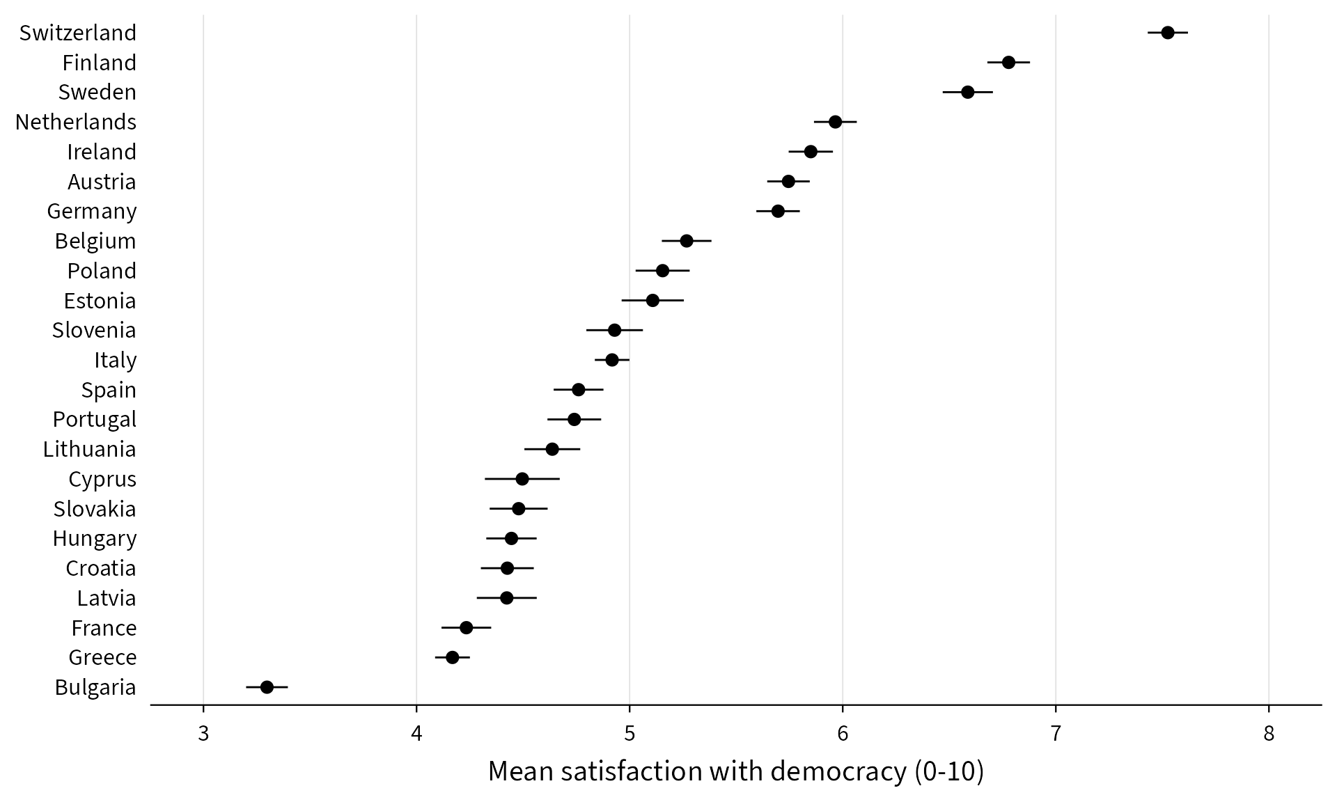
Figure: Mean satisfaction with democracy by country, with 95% confidence intervals. Data: European Social Survey, round 11 (unweighted).
Pretty regression tables
| (1) | (2) | |
|---|---|---|
| * p < 0.1, ** p < 0.05, *** p < 0.01 | ||
| OLS. Dependent variable: left-right self-placement (0 = left, 10 = right). Standard errors in parentheses. | ||
| Age (years) | 0.003*** | 0.003*** |
| (0.001) | (0.001) | |
| Woman | -0.302*** | -0.326*** |
| (0.024) | (0.024) | |
| Education (years) | -0.030*** | -0.027*** |
| (0.003) | (0.003) | |
| Observations | 33,945 | 33,945 |
| R² | 0.009 | 0.033 |
| Country fixed effects | No | Yes |
Made with the modelsummary package, which also writes Word and LaTeX tables.
Tuesday
Expect the steps from the labs, applied to variables you haven’t seen: inspect, clean, check, describe, test, model, and interpret each result in your own words.
To keep learning (all free online): Hands-On Programming with R for R itself, then R for Data Science for data analysis, and the Posit cheat sheets.
Appendix: Every Lab Function
Start and import
| Function | What it does | Example from the labs | Watch out |
|---|---|---|---|
install.packages() |
downloads a package, once per computer | install.packages("car") |
in the console, not in the exam script |
library() |
loads a package for this session | library(car) |
every session; the stats package is always loaded |
getwd() |
shows the working directory | getwd() |
with a project it’s the project folder |
list.files() |
lists the files in a folder | list.files("data") |
the exact file name to use |
read.csv() |
imports a comma-separated file | read.csv("data/ess.csv") |
path relative to the project |
read.csv2() |
imports a semicolon-separated file | read.csv2("students.csv") |
use one of the two, not both |
names() |
the variable names | names(dataset) |
|
dim(), nrow()
|
rows × columns | dim(dataset) |
rows = respondents |
head() |
the first rows | head(dataset) |
|
str() |
the type of each variable | str(dataset) |
chr = text, int/num = numbers |
Inspect and clean
| Function | What it does | Example from the labs | Watch out |
|---|---|---|---|
table() |
counts each value | table(dataset$V242065) |
add useNA = "ifany" to see NA
|
summary() |
min, quartiles, mean, max | summary(dataset$agea) |
a max of 999 is a code |
unique(), sort()
|
the distinct values | sort(unique(dataset$lrscale)) |
|
ifelse() |
if-then for every row | ifelse(x %in% c(77, 88, 99), NA, x) |
ifelse(condition, yes, no) |
%in% |
“is one of” | x %in% c(1, 2, 3) |
|
==, !=, >=, &, |
|
compare, AND, OR | x >= 0 & x <= 10 |
== compares, = sets an argument |
NA |
missing value | ifelse(..., x, NA) |
no quotes: "NA" is text |
is.na() |
TRUE where missing | sum(is.na(dataset$age)) |
x == NA doesn’t work |
x[condition] <- value |
change only the matching rows | d$cat[d$x <= 3] <- 1 |
Lab 5’s 3-category recode |
factor() |
treat numbers as categories | factor(gndr) |
first level = reference |
subset() |
keep the matching rows | subset(dataset, cntry == "FR") |
text needs quotes |
mutate() + case_when()
|
dplyr recode | Lab 3 solution | needs library(dplyr)
|
Describe and compare
| Function | What it does | Example from the labs | Watch out |
|---|---|---|---|
mean(), median(), sd()
|
centre, spread | mean(x, na.rm = TRUE) |
without na.rm → NA
|
prop.table() |
turns counts into proportions | prop.table(table(x, y), 1) * 100 |
1 = row %, 2 = column % |
round() |
rounds | round(x, 1) |
halves round to even |
hist() |
histogram | hist(dataset$like_democrat) |
for a 0 to 10 scale: breaks = seq(-0.5, 10.5, 1)
|
barplot() |
bar chart of counts | barplot(table(x)) |
|
boxplot() |
distribution by group | boxplot(swd ~ voted_2024, data = d) |
|
plot() |
scatter plot | plot(d$age, d$like_democrat) |
x first, then y |
aggregate() |
statistic by group | aggregate(y ~ group, data = d, FUN = mean) |
drops NA itself |
cor() |
correlation r | cor(x, y, use = "complete.obs") |
no p-value: cor.test()
|
t.test() |
difference of two means | t.test(y ~ group, data = d) |
the group needs exactly 2 values |
chisq.test() |
association of two categorical variables | chisq.test(table(x, y)) |
no direction: look at the % |
Models
| Function | What it does | Example from the labs | Watch out |
|---|---|---|---|
lm() |
linear regression (OLS) | lm(y ~ age + factor(gndr) + edu, data = d) |
factor() for categories |
summary(model) |
coefficients, p-values, R² | summary(model1) |
note how many rows were deleted |
confint() |
95% confidence intervals | confint(model1) |
|
nobs() |
rows the model used | nobs(model1) |
|
coef() |
the coefficients as numbers | coef(m)["edu"] |
for interaction arithmetic |
glm(…, family = binomial) |
logistic regression | glm(far_right ~ …, family = binomial) |
only the sign of the coefficients |
margins() |
average marginal effects | summary(margins(logit1)) |
× 100 = percentage points |
multinom() |
multinomial logit | multinom(y3 ~ …, data = d) |
reference = first level; library(nnet)
|
x1 * x2 |
interaction | factor(gndr) * eduyrs |
slope for group 2 = b_x + b_int
|
bptest() |
Breusch-Pagan test | bptest(model2) |
H0: homoskedasticity; library(lmtest)
|
vif() |
multicollinearity | vif(model2) |
below 10: not a concern; library(car)
|
plot(fitted, resid) + abline(h = 0)
|
residual plot | plot(m$fitted.values, m$residuals) |
look for a spread that changes |
Quantitative Methods I · Quick R Recap